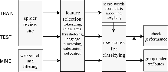
Figure 1: Overview of project architecture and flow.
Product reviews exist in a variety of forms on the web: sites dedicated to a specific type of product (such as MP3 player or movie pages), sites for newspapers and magazines that may feature reviews (like Rolling Stone or Consumer Reports), sites that couple reviews with commerce (like Amazon), and sites that specialize in collecting professional or user reviews in a variety of areas (like C|net or ZDnet in electronics, or the more broad Epinions.com and Rateitall.com). Less formal reviews are available on discussion boards and mailing list archives, as well as in Usenet via Google Groups. Users also comment on products in their personal web sites and blogs, which are then aggregated by sites such as Blogstreet.com, AllConsuming.net, and onfocus.com. When trying to locate information on a product, a general web search turns up several useful sites, but getting an overall sense of these reviews can be daunting or time-consuming.
In the movie review domain, sites like Rottentomates.com have sprung up to try to impose order on the void, providing ratings and brief quotes from numerous reviews and generating an aggregate opinion. Such sites even have their own category--"Review Hubs"--on Yahoo!
On the commerical side, Internet clipping services like Webclipping.com, eWatch.com, and TracerLock.com watch news sites and discussion areas for mentions of a given company or product, trying to track "buzz." Print clipping services have been providing competitive intelligence for some time. The ease of publishing on the web has led to an explosion in content to be surveyed, but the same technology makes automation much more feasible.
This paper describes a tool for sifting through and synthesizing product reviews, automating the sort of work done by aggregation sites or clipping services. We begin by using structured reviews for testing and training, identifying appropriate features and scoring methods from information retrieval for determining whether reviews are positive or negative. These results perform as well as traditional machine learning methods. We then use the classifier to identify and classify review sentences from the web, where classification is more difficult. However, a simple technique for identifying the relevant attributes of a product produces a subjectively useful summary.
Although the broad problem we are trying to solve is unique in the literature, there are various relevant areas of existing research. Separating reviews from other types of web pages about a product is similar to other style classification problems. Trying to determine the sentiment of a review has been attempted in other applications. Both of these tasks draw on work done finding the semantic orientation of words.
The task of separating reviews from other types of content is a genre or style classification problem. It involves identifying subjectivity, which Finn et al. [2] attempted to do on a set of articles spidered from the web. A classifier based on the relative frequency of each part of speech in a document outperformed bag-of-words and custom-built features.
But determining subjectivity can be, well, subjective. Wiebe et al. [25] studied manual annotation of subjectivity at the expression, sentence, and document level and showed that not all potentially subjective elements really are, and that readers' opinions vary.
Trying to understand attributes of a subjective element--such as whether it is positive or negative (polarity or semantic orientation) or has different intensities (gradability)--is even more difficult. Hatzivassiloglou and McKeown [4] used textual conjunctions such as "fair and legitimate" or "simplistic but well-received" to form clusters of similarly- and oppositely-connoted words. Other studies showed that restricting features used for classification to those adjectives that come through as strongly dynamic, gradable, or oriented improved performance in the genre-classification task [5,24].
Turney and Littman [23] determined the extent of similarity between two words by counting the number of results returned by web searches joining the words with the NEAR operator. The relationship between an unknown word and a set of manually-selected seeds was used to place it into a positive or negative subjectivity class.
This area of work is related to the general problem of word clustering. Lin [8] and Pereira et al. [16] used linguistic colocations to group words with similar uses or meanings.
One interesting approach to classifying sentiment uses fuzzy logic. Subasic and Huettner [20] manually constructed a lexicon associating words with affect categories, specifying an intensity (strength of affect level) and centrality (degree of relatedness to the category). For example, "mayhem" would belong, among others, to the category violence with certain levels of intensity and centrality. Fuzzy sets are then used to classify the affect of a document.
Another technique uses a manually-constructed lexicon to derive global directionality information (e.g. "Is the agent in favor of, neutral or opposed to the event?") which converts linguistic pieces into roles in a metaphoric model of motion, with labels like BLOCK or ENABLE [6].
Recently, Liu et al. [10] used relationships from the Open Mind Commonsense database and manually-specified ground truth to assign scalar affect values to linguistic features. These corresponded to six basic emotions (happy, sad, anger, fear, disgust, surprise). Several techniques were applied to classify passages using this knowledge, and user studies were conducted with an email composer that presented face icons corresponding to the inferred emotion.
At a more applied level, Das and Chen [1] used a classifier on investor bulletin boards to see if apparently positive postings were correlated with stock price. Several scoring methods were employed in conjunction with a manually crafted lexicon, but the best performance came from a combination of techniques. Another project, using Usenet as a corpus, managed to accurately determine when posters were recommending a URL in their message [21].
Recently, Pang et al. [14] attempted to classify movie reviews posted to Usenet, using accompanying numerical ratings as ground truth. A variety of features and learning methods were employed, but the best results came from unigrams in a presence-based frequency model run through Support Vector Machines (SVMs), with 82.9 percent accuracy. Limited tests on this corpus (available at http://www.cs.cornell.edu/people/pabo/movie-review-data/) using our own classifier yielded only 80.6 percent accuracy using our baseline bigrams method. As we discuss later, comparisons are less clear-cut on our own corpus. We believe this is due to differences in the problems we are studying; among other things, the messages in our corpus are smaller and cover a different domain.
Two commercial solutions to opinion mining use proximity measures and word lists to fit data into templates and construct models of user opinion. The first is from Opion, now part of Planetfeedback.com [7,22]. The second is from NEC Japan [13].
Finally, there is much relevant work in the general area of information extraction and pattern-finding for classification. One technique uses linguistic units called relevancy signatures as part of CIRCUS, a tool for sorting documents [19].
Our approach, as shown in Figure 1, begins with training a classifier using a corpus of self-tagged reviews available from major web sites. We then refine our classifier using this same corpus before applying it to sentences mined from broad web searches.
Figure 1: Overview of project architecture and flow.
User reviews from large web sites where authors provide quantiative or binary ratings are perfect for training and testing a classifier for sentiment or orientation. The range of language used in such corpora is exactly what we want to focus our future mining efforts on. The two sites we chose were C|net and Amazon, based on the number of reviews, number of products, review quality, available metadata, and ease of spidering.
C|net allows users to input a text review, a title, and a thumbs-up or thumbs-down rating. Additional data available but not used in this project include date and time, author name, and ratings from 1-5 for "support", "value", "quality", and "features." A range of computer and consumer electronics products were chosen arbitrarily from those available, providing a diverse but constrained set of documents, as shown in Table 1. Editorial reviews by C|net's writers were not included in the corpus.
Amazon, meanwhile, has one scalar rating per product (number of stars), enabling more precise training, and tends to have longer reviews, which are easier to classify. Unfortunately, electronics products generally have fewer reviews than at C|net, visible in Table 2. Reviews of movies, music and books were more plentiful, but attempting to train classifiers for these more subjective domains is a more difficult problem. One reason for this is that review-like terms are often found in summaries (e.g. "The character finds life boring." vs. "This book is boring.").
Table 1: Breakdown of C|net categories.
Positive reviews are ones marked by their authors with a "thumbs-up", negative reviews are those given a "thumbs-down". (Numbers are restricted to unique reviews containing more than 1 token.)
| Reviews | |||
|---|---|---|---|
| C|net category | Products | Pos. | Neg. |
| Networking kits | 13 | 191 | 144 |
| TVs | 143 | 743 | 119 |
| Laser printers | 74 | 1,088 | 439 |
| Cheap laptops | 147 | 3,057 | 683 |
| PDAs | 83 | 3,335 | 896 |
| MP3 players | 118 | 5,418 | 2,108 |
| Digital cameras | 173 | 12,078 | 1,275 |
Table 2: Breakdown of Amazon categories.
We arbitrarily consider positive reviews to be those where authors give a score of 3 stars or higher out of 5. (Numbers are restricted to unique reviews containing more than 1 token.)
| Reviews | |||
|---|---|---|---|
| Amazon category | Products | Pos. | Neg. |
| Entertainment laptops | 29 | 110 | 29 |
| MP3 players | 201 | 979 | 411 |
| PDAs | 169 | 842 | 173 |
| Top digital cameras | 100 | 1,410 | 251 |
| Top books | 100 | 578 | 120 |
| Alternative Music | 25 | 210 | 7 |
| Top movies | 100 | 719 | 81 |
Two tests were decided on. Test 1 tests on each of the 7 C|net categories in turn, using the remaining 6 as a training set, and takes the macroaverage of these results. This evaluates the ability of the classifier to deal with new domains and retains the skews of the original corpus. There are five times as many positive reviews as negative ones, and certain products have many more reviews: MP3 players have 13,000 reviews, but networking kits have only 350. Half of the products have fewer than 10 reviews, and a fifth of the reviews have fewer than 10 tokens. Additionally, there are some duplicate or near-duplicate reviews, including one that had been posted 23 times.
Test 2 used 10 randomly selected sets of 56 positive and 56 negative reviews from each of the 4 largest C|net categories, for a total of 448 reviews per set. Each review in the test was unique and had more than ten tokens. Using one set for testing and the remainder for training, we conducted 10 trials and took their average. This was a much cleaner test of how well the classifier classified the domains it had learned.
Although there are various ways of breaking down classification performance--such as precision and recall--and weighting performance--using values like document length or confidence--these values did not seem to provide any better differentiation than simple accuracy.
Our baseline algorithm is described in Sections 3.6 and 3.8. In the remainder of this section, we examine the efficacy of introducing a number of more sophisticated strategies.
Starting with a raw document (a portion of a web page in testing and training, and a complete web page for mining), we strip out HTML tags and separate the document into sentences. These sentences are optionally run through a parser before being split into single-word tokens. A variety of transformations can then be applied to this ordered list of lists.
One problem with many features is that they may be overly specific. For example, "I called Nikon" and "I called Kodak" would ideally be grouped together as "I called X." Substitutions have been used to solved exactly these sorts of problems in subjectivity identification, text classification, and question answering [18,19,26], but, as indicated in Table 3, they are mostly ineffective for our task.
We begin by replacing any numerical tokens with NUMBER. although this does not have a significant net effect on performance, it helps eliminate misclassifications where a stand-alone number like "64" carries a strong positive weight from appearing in strings like "64 MB."
In some cases, we find a second substitution to be helpful. all instances of a token from the product's name, as derived from the crawler or search string, are replaced by _productname. This produces the desired effect in our "I called X" example.
Two additional substitutions were considered. The first occurs in a global context, replacing low-frequency words that would otherwise be thresholded out with _unique. Thus, in an actual example from camera reviews, "peach fuzz" and "pollen fuzz" become "_unique fuzz." This substitution degraded performance, however, apparently due to overgeneralization.
The other replaces words that seem to occur only in certain product categories with _producttypeword. Thus, "the focus is poor" and "the sound is poor" could be grouped in a general template for criticism. However, finding good candidates for replacement is difficult. Our first attempt looked for words that were present in many documents but almost exclusively in one category. Something like "color," which might occur in discussions of both digital cameras and PDA's would not be found by this method. A second try looked at the information gain provided by a given word when separating out categories. Neither yielded performance improvements.
Table 3: Results of using substitutions to generalize over distracting words in different scopes, compared to n-gram baselines.
Rare words were replaced globally, domain-specific words were replaced for categories, and product names were replaced for products. The table is sparse because no suitable method for finding category substitutions was available for Test 2. In all cases, we substitute NUMBER for numbers. The one statistically significant substitution is in bold (t=2.448).
| Substitutions | Bigrams | Trigrams | ||||
|---|---|---|---|---|---|---|
| Global | Cat. | Prod. | Test 1 | Test 2 | Test 1 | Test 2 |
| 88.3% | 84.6% | 88.7% | 84.5% | |||
| Y | 88.3% | 84.7% | 88.4% | 84.2% | ||
| Y | 88.3% | 88.8% | 84.2% | |||
| Y | 88.2% | 84.7% | 88.9% | 84.6% | ||
| Y | Y | 88.3% | 88.7% | |||
| Y | Y | Y | 88.3% | |||
At this point, we can pass our document through Lin's MINIPAR linguistic parser (available at http://www.cs.ualberta.ca/~lindek/minipar.htm) sentence by sentence, yielding the part of speech of each word and the relationships between parts of the sentence. This computationally-expensive operation enables some interesting features, but unfortunately none of them improve performance on our tests, as shown in Table 4.
Knowing the part of speech, we can run words through WordNet, a database for finding similarities of meaning (available at http://www.cogsci.princeton.edu/~wn/). But, like any such tool, it suffers from our inability to provide word sense disambiguation. Because each word has several meanings, it belongs to several synsets. Lacking any further information, we make a given instance of the word an equally-likely member of each of them. Unfortunately, this can produce more noise than signal. False correlations can occur, such as putting "duds" and "threads" together, even though in the context of electronics reviews neither refers to clothing. Furthermore, the use of WordNet can cause feature sets to grow to unmanageable size. Attempts to develop a custom thesaurus from word colocations in the corpus were equally unsuccessful.
Used directly, colocations produce an effect opposite that of WordNet. Triplets of the form Word(part-of-speech):Relation:Word(part-of-speech) can qualify a term's occurrence. This seems like it would be particularly useful for pulling out adjective-noun relationships since they can occur several words apart, as in "this stupid ugly piece of garbage" (stupid(A):subj:piece(N)) or as part of a modal sentence as in "this piece of garbage is stupid and ugly" (piece(N):mod:ugly(A)). However, using colocations as features, even after putting noun-adjective relationships into a canonical form, was ineffective.
Two less costly attempts to overcome the variations and dependencies in language were also tried with limited success.
Stemming removes suffixes from words, causing different forms of the same word to be grouped together. When Porter's stemmer [17] was applied, our classifier performed below the baseline in Test 1, but better in Test 2. Again, the problem seems to be overgeneralization. The corpus of reviews is highly sensitive to minor details of language, and these may be glossed over by the stemmer. For example, negative reviews tend to occur more frequently in the past tense, since the reviewer might have returned the product.
We then tried to identify negating phrases such as "not" or "never" and mark all words following the phrase as negated, such as turning "not good or useful" into "NOTgood NOTor NOTuseful." While Pang noted a slight improvement from this heuristic, our implementation only hurt performance. It may be that simple substrings do a more accurate job of capturing negated phrases.
Table 4: Results of linguistic features.
| Features | Test 1 | Test 2 |
|---|---|---|
| Unigram baseline | 84.9% | 82.2% |
| WordNet | 81.5% | 80.2% |
| Colocation | 83.3% | 77.3% |
| Stemming | 84.5% | 83.0% (t=3.787) |
| Negation | 81.9% | 81.5% |
Once tokenization and substitution are complete, we can combine sets
of ![]() adjacent tokens into
adjacent tokens into ![]() -grams, a standard technique in
language processing. For example, "this" followed by "is" becomes
"this is" in a bigram. Examples of high-scoring n-grams are shown in
Table 5, and performance results are shown in Table
3. In our task, n-grams proved quite
powerful. In Test 1, trigrams performed best, while in Test 2, bigrams
did marginally better. Including lower-order features (e.g. including
unigrams with bigrams) degraded performance unless these features had
smaller weights (as little as a quarter of the weight of the larger
features). Experiments using lower-order features for smoothing when a
given higher-order feature had not been present in the training set
also proved unsuccessful.
-grams, a standard technique in
language processing. For example, "this" followed by "is" becomes
"this is" in a bigram. Examples of high-scoring n-grams are shown in
Table 5, and performance results are shown in Table
3. In our task, n-grams proved quite
powerful. In Test 1, trigrams performed best, while in Test 2, bigrams
did marginally better. Including lower-order features (e.g. including
unigrams with bigrams) degraded performance unless these features had
smaller weights (as little as a quarter of the weight of the larger
features). Experiments using lower-order features for smoothing when a
given higher-order feature had not been present in the training set
also proved unsuccessful.
A related technique simulates a NEAR operator by putting
together words that occur within ![]() words of each other into a single
feature. While improving performance, this was not as effective as
trigrams. Somewhat similar effects are produced by allowing wildcards
in the middle of n-gram matches.
words of each other into a single
feature. While improving performance, this was not as effective as
trigrams. Somewhat similar effects are produced by allowing wildcards
in the middle of n-gram matches.
Table 5: N-gram features from C|net with highest information gain.
Note how the dominance of positive camera reviews skews the global features. "." is the end-of-sentence marker.
| Unigrams | Bigrams | Trigrams | Distance 3 |
|---|---|---|---|
| Top positive features | |||
| great | easy to | easy to use | . great |
| camera | the best | i love it | easy to |
| best | . great | . great camera | camera great |
| easy | great camera | is the best | best the |
| support | to use | . i love | . not |
| excellent | i love | first digital camera | easy use |
| back | love it | for the price | .camera |
| love | a great | to use and | i love |
| not | this camera | is a great | to use |
| digital | digital camera | my first digital | camera this |
| Top negative features | |||
| waste | returned it | taking it back | return to |
| tech | after NUMBER | time and money | customer service |
| sucks | to return | it doesn't work | poor quality |
| horrible | customer service | send me a | . returned |
| terrible | . poor | what a joke | the worst |
| return | the worst | back to my | i returned |
| worst | back to | . returned it | support tech |
| customer | tech support | . why not | not worth |
| returned | not worth | something else . | . poor |
| poor | it back | . the worst | back it |
Noting the varied benefits of n-grams, we developed an algorithm that attempts to identify arbitrary-length substrings that provide "optimal" classification. We are faced with a tradeoff: as substrings become longer and generally more discriminatory, their frequency decreases, so there is less evidence for considering them relevant. Simply building a tree of substrings up to a cutoff length, treating each sufficiently-frequent substring as relevant, yields no better than 88.5 percent accuracy on the first test using both our baseline and Naive Bayes.
A more complicated approach, which compares each node on the tree to its children to see if its evidence-differentiation tradeoff is better than its child, sometimes outperforms n-grams. We experimented with several criteria for choosing not to pursue a subtree any further, including its information gain relative to the complete set, the difference between the scores that would be given to it and its parent, and its document frequency. We settled on a threshold for information gain relative to a node's parent. A second issue involved how these features would actually be assigned scores. Results from different feature schemes are shown in Table 6. Ways of then matching testing data to the scored features are discussed later.
To improve performance, we drew on Church's suffix array algorithm [27]. Future work might incorporate techniques from probabilistic suffix trees [15].
Table 6: Results of some scoring metrics for variable-length substrings.
Intensity is
![]() , df is
document frequency, len is substring length.
, df is
document frequency, len is substring length.
| Scoring method | Test 1 | Test 2 |
|---|---|---|
| Trigram baseline | 88.7% | 84.5% |
| int | 87.7% | 84.9% |
| int * df | 87.8% | 85.1% (t=2.044) |
| int * df * len | 86.0% | 84.2% |
| int * log(df) | 62.8% | 77.0% |
| int | 58.3% | 77.3% |
| int * len | 87.0% | 83.9% |
| int * log(df) * len | 60.3% | 77.8% |
| int * df * log(len) | 80.0% | 81.0% |
Our features complete, we then count their frequencies--the number of times each term occurs, the number of documents each term occurs in, the number of categories a term occurs in, and the number of categories a term occurs in. To overcome the skew of Test 1, we can also normalize the counts. We then set upper and lower limits for each of these measures, constraining the number of features we look at. This improves relevance of the remaining features and reduces the amount of required computation. In some applications, dimensionality reduction is accomplished by vector methods such as SVD or LSI. However, it seemed that doing so here might remove minor but important features.
Results are shown in Table 7. although not providing the highest possible accuracy, our default was to only use terms appearing in at least 3 documents so that the term space was greatly reduced. although some higher thresholds show better results, this is deceptive; some documents that were being misclassified now have no known features and are ignored during classification. Attempts to normalize the values used as document frequencies in thresholding did not help, apparently because the testing set had the same skew the training set did. The need for such a low threshold also points to the wide variety of language employed in these reviews and the need to maximize the number of features we capture, even with sparse evidence.
Table 7: Results of thresholding schemes on baseline performance.
all defaults are 1, except for a minimum document frequency of 3.
| Base freq. | Value | Test 1 | Test 2 |
|---|---|---|---|
| Unigram baseline | 85.0% | 82.2% | |
| product | 2 | 84.9% | 82.2% |
| product | 3 | 85.1% | 82.2% |
| product | 4 | 85.0% | 82.1% |
| product | 7 | 84.9% | 82.4% |
| product | 10 | 84.4% | 82.2% |
| document | 1 | 85.3% | 82.0% |
| document | 2 | 85.1% | 82.3% |
| document | 5 | 85.0% | 82.3% |
| document | 10 | 84.7% | 82.0% |
| product type | 2 | 84.9% | 82.2% |
| product type | 4 | 85.0% | 82.3% |
| product type | 5 | 84.9% | 82.3% |
| max. document | .50 | 83.9% | 82.6% (t=1.486) |
| max. document | .75 | 84.9% | 82.2% |
| max. document | .25 | 82.1% | 81.5% |
Before assigning scores based on term frequencies, we can try smoothing these numbers, assigning probabilities to unseen events and making the known probabilities less "sharp." although not helpful for our baseline metric, improvements were seen with Naive Bayes.
The best results came from Laplace smoothing, also known as
add-one. We add one to each frequency, making the frequency of a
previously-unseen word non-zero. We adjust the denominator
appropriately. Therefore,
![]() where
where ![]() is the number of unique words.
is the number of unique words.
Two other methods were also tried. The Witten-Bell method takes
![]() , where
, where ![]() is the number of tokens observed, and
assigns that as the probability of an unknown word, reassigning the
remaining probabilities proportionally.
is the number of tokens observed, and
assigns that as the probability of an unknown word, reassigning the
remaining probabilities proportionally.
Good-Turing, which did not even do as well as Witten-Bell, is more
complex. It orders the elements by their ascending frequencies ![]() ,
and assigns a new probability equal to
,
and assigns a new probability equal to ![]() where
where
![]() and
and ![]() is the number of features having
frequency
is the number of features having
frequency ![]() . The probability of an unseen element is equal to the
probability of words that were seen only once, i.e.
. The probability of an unseen element is equal to the
probability of words that were seen only once, i.e.
![]() . Because some values of
. Because some values of ![]() are unusually
low or high in our sample, pre-smoothing is required. We
utilized the Simple Good-Turing code from Sampson where the values are
smoothed with a log-linear curve [3]. We also used
add-one smoothing so that all frequencies were non-zero; this worked
better than using only those data points that were known.
are unusually
low or high in our sample, pre-smoothing is required. We
utilized the Simple Good-Turing code from Sampson where the values are
smoothed with a log-linear curve [3]. We also used
add-one smoothing so that all frequencies were non-zero; this worked
better than using only those data points that were known.
After selecting a set of features ![]() and optionally smoothing their
probabilities, we must assign them scores, used to place test documents in the set of positive reviews
and optionally smoothing their
probabilities, we must assign them scores, used to place test documents in the set of positive reviews ![]() or negative reviews
or negative reviews ![]() . We tried some
machine-learning techniques using the Rainbow text-classification
package [9], but Table
9 shows the performance was no better
than our method.
. We tried some
machine-learning techniques using the Rainbow text-classification
package [9], but Table
9 shows the performance was no better
than our method.
We also tried SVM![]() (available at http://svmlight.joachims.org),
the package used by Pang et al. When duplicating their methodology (normalizing, presence model, feature space constraining), the SVM outperformed our
baseline metric on Test 2 but underperformed it on Test 1, as shown in
Table 8. Furthermore, our best scoring
result using simple bigrams on Test 2, the odds ratio metric, has an
accuracy of 85.4%, statistically indistinguishable from the SVM
result (t=.527).
(available at http://svmlight.joachims.org),
the package used by Pang et al. When duplicating their methodology (normalizing, presence model, feature space constraining), the SVM outperformed our
baseline metric on Test 2 but underperformed it on Test 1, as shown in
Table 8. Furthermore, our best scoring
result using simple bigrams on Test 2, the odds ratio metric, has an
accuracy of 85.4%, statistically indistinguishable from the SVM
result (t=.527).
On the other hand, our implementation of Naive Bayes with Laplace
smoothing does better on Test 1 for unigrams, but worse on Test 2 and
when bigrams are used. The results are shown in Table
10. To prevent underflow, the implementation
used the sum of ![]() s, yielding the document score formula below.
s, yielding the document score formula below.
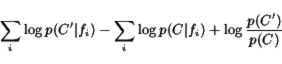
Table 8: Results from SVM![]() .
.
For bigrams on Test 1, a polynomial kernel was used, all other settings were defaults.
| Test 1 | Test 2 | |||
|---|---|---|---|---|
| Method | Unigrams | Bigrams | Unigrams | Bigrams |
| Baseline | 85.0% | 88.3% | 82.2% | 84.6% |
| SVM | 81.1% | 87.2% | 84.4% | 85.8% |
Table 9: Results of machine learning using Rainbow.
| Method | Test 2 |
|---|---|
| Unigram baseline | 82.2% |
| Maximum entropy | 82.0% |
| Expectation maximization | 81.2% |
Table 10: Results of tests using Naive Bayes.
| Method | Test 1 | Test 2 |
|---|---|---|
| Unigram baseline | 84.9% | 82.2% |
| Naive Bayes | 77.0% | 80.1% |
| NB w/ Laplace | 87.0% (t=2.486) | 80.1% |
| NB w/ Witten-Bell | 83.1% | 80.3% |
| NB w/ Good-Turing | 76.8% | 80.1% |
| NB w/ Bigrams + Lap | 86.9% | 81.9% |
We obtain more consistent performance across tests with less computation when we use the various calculated frequencies and techniques from information retrieval, which we compare in Table 11. Our scoring method, which we refer to as the baseline, was fairly simple.
We determine
![]() , the normalized term frequency, by taking the number of
times a feature
, the normalized term frequency, by taking the number of
times a feature ![]() occurs in
occurs in ![]() and dividing it by the total
number of tokens in
and dividing it by the total
number of tokens in ![]() . A term's score is thus a measure of bias
ranging from –1 to 1.
. A term's score is thus a measure of bias
ranging from –1 to 1.
Several alternatives fail to perform as well. For example, we can use
the total number of terms remaining after thresholding as the
denominator in calculating ![]() , which makes each value
larger. This improves performance on Test 2, but not on Test 1. Or we
can completely redefine the event model for
, which makes each value
larger. This improves performance on Test 2, but not on Test 1. Or we
can completely redefine the event model for ![]() , making it use
presence and document frequency instead of term frequency. Here, we
take the number of documents
, making it use
presence and document frequency instead of term frequency. Here, we
take the number of documents ![]() occurs in from
occurs in from ![]() divided by the
number of documents in
divided by the
number of documents in ![]() . This performs better on Test 2 but does
worse as a result of the skew in Test 1.
. This performs better on Test 2 but does
worse as a result of the skew in Test 1.
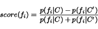
A similar measure, the odds ratio [11] is calculated as
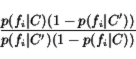
Although discussed as a method for thresholding features prior to machine learning, we found that it does well on Test 2 as an actual score assignment, performing on par with SVMs. Unfortunately, this metric is sensitive to differences in class sizes, and thus performs poorly on Test 1. When using term instead of document probabilities, performance is more consistent, but worse than our measure.
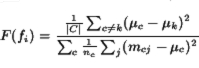
Other measures did poorly on both tests. One option was the Fisher
discriminant, which looks at the differences in the average term
frequency of a word in different classes, normalized by the term's
intra-class variance. If
![]() , and
, and ![]() is the
average term frequency of
is the
average term frequency of ![]() in class
in class ![]() , and
, and ![]() is the
count of
is the
count of ![]() in message
in message ![]() of class
of class ![]() ,
,
But this measure is not well-suited to the noisy, binary classification problem we are confronted with.
A second method used information theory to assign each feature a score. As in the failure of reweighting, it may be that these methods are simply too sensitive to term frequency when simple absence or presence is more important. The definition of entropy for a binary classification is
![]()
Information gain is calculated as
![]()
where each event is a document. Words are assigned a sign based on which class had the highest normalized term frequency.
We also tried using Jaccard's measure of similarity as an
ultra-simple benchmark, which takes the number of words ![]() has in
common with
has in
common with ![]() , divided by the number of words in
, divided by the number of words in ![]() . But
this works quite poorly due to the skew in the data set. We also
found that setting
. But
this works quite poorly due to the skew in the data set. We also
found that setting
![]() produced accuracy below simply assigning everything to
the positive set.
produced accuracy below simply assigning everything to
the positive set.
Table 11: Results of alternative scoring schemes.
| Features | Test 1 | Test 2 |
|---|---|---|
| Unigram baseline | 85.0% | 82.2% |
| all positive baseline | 76.3% | 50.0% |
| Odds ratio (presence model) | 53.3% | 83.3% (t=3.553) |
| Odds ratio | 84.7% | 82.6% |
| Probabilities after thresholding | 76.3% | 82.7% (t=2.474) |
| Baseline (presence model) | 59.8% | 83.1% (t=3.706) |
| Fisher discriminant | 76.3% | 56.9% |
| Counting | 75.5% | 73.2% |
| Information gain | 81.6% | 80.6% |
One interesting property of the baseline measure is that it does not incorporate the strength of evidence for a given feature. Thus, a rare term, like "friggin", which occurs in 3 negative documents in one set, has the same score, –1, as "livid", which occurs 23 times in the same set. Table 12 shows that most attempts to incorporate weighting were unsuccessful.
Although information retrieval traditionally utilizes inverse document
frequency (IDF) to help identify rare words which will point to
differences between sets, this does not make sense in
classification. Multiplying by document frequency, dampened by
![]() , did provide better results on Test 1.
, did provide better results on Test 1.
We tried assigning weights using a Gaussian weighting scheme, where weights decrease polynomially with distance from a certain mean frequency. This decreases the importance of both infrequent and too-frequent terms. Though the mean and variance must be picked arbitrarily (since the actual frequencies are in a Zipf distribution), some of the parameters we tried seemed to work.
We also tried using the residual inverse document frequency as
described by Church, which looks at the difference between the IDF and
the IDF predicted by the Poisson model for a random word (i.e. ![]() ). However, no improvements
resulted.
). However, no improvements
resulted.
Table 12: Results of weighting schemes.
Mean and deviation for Gaussian listed in parentheses.
| Base freq. | Transform | Test 1 | Test 2 |
|---|---|---|---|
| Unigram baseline | 85.0% | 82.2% | |
| document | 81.1% | 65.4% | |
| document | log | 85.5% (t=1.376) | 81.6% |
| document | sqrt | 85.3% | 77.4% |
| document | inverse | 84.7% | 79.7% |
| document | normalized | 82.0% | 65.4% |
| document | log norm. | 84.7% | 81.7% |
| term | 84.9% | 82.2% | |
| term | log | 84.9% | 82.2% |
| term | gauss (3,.5) | 85.7% (t=2.525) | 81.7% |
| product | 85.6% | 77.6% | |
| product | log | 85.0% | 80.7% |
| product type | 84.7% | 65.4% | |
| product type | sqrt | 84.8% | 82.2% |
| document + term | ridf | 82.2% | 80.8% |
| Bigram baseline | 88.3% | 84.6% | |
| bigram term | gauss (4,.5) | 88.3% | 84.6% |
| bigram doc. | log | 88.4% | 84.3% |
Once each term has a score, we can sum the scores of the words in
an unknown document and use the sign of the total to determine a
class. In other words, if document ![]() ,
,
where
When we have variable-length features from our substring tree, there are several options for choosing matching tokens. The most effective technique is to find the longest possible feature matches starting at each token. although it appears this may lead longer features to carry more weight (e.g. "I returned this" will be counted again as "returned this"), this turns out to not be a problem since the total score is still linear in the number of tokens. When we tried disallowing nested matches or using dynamic programming to find the highest-confidence non-overlapping matches, the results were not as good. We also experimented with allowing wildcards in the middle of tokens.
One trick tried during classification was a sort of bootstrapping, sometimes called transductive learning. As the test set was classified, the words in the test set were stored and increasingly used to supplement the scores from the training set. However, no method of weighting this learning seemed to actually improve results. At best, performance was the same as having no bootstrapping at all.
In our preliminary work with the Amazon corpus, different techniques were needed. The intuitive approach was to give each word a weight equal to the average of the scores of the documents it appears in. Then we could find the average word score in a test document in order to predict its classification. In practice, this tends to cluster all of the documents in the center. Trying to assign each word a score based on the slope of the best fit line along its distribution had the same result.
Two solutions to this problem were tried: exponentially "stretching" the assigned score using its difference from the mean, and thresholding the feature set so only those with more extreme scores were included. Both worked moderately well, but a Naive Bayes classification system, with separate probabilities maintained for each of the 5 scoring levels, actually worked even better.
Of course, the absolute classification is only one way of evaluating performance, and ideally a classifier should get more credit for mis-rating a 4 review as a 5 than as a 1, analogous to confidence weighting in the binary classification problem.
Mooney et al. [12] faced a similar problem when trying to use Amazon review information to train book recommendation tools. They used three variations: calculating an expected value from Naive Bayes output, reducing the classification problem to a binary problem, and weighting binary ratings based on the extremity of the original score.
As a follow-on task, we crawl search engine results for a given product's name and attempt to identify and analyze product reviews within this set. Initially, we use a set of heuristics to discard some pages, paragraphs, and sentences that are unlikely to be reviews (such as pages without "review" in their title, paragraphs not containing the name of the product, and excessively long or short sentences). We then use the classifiers trained on C|net to rate each sentence in each page. We hoped that the features from the simple classification problem would be useful, although the task and the types of documents under analysis are quite different.
In fact, the training results give us some misdirection: negatively weighted features can be anything from "headphones" (not worth mentioning if they are okay) to "main characters" (used only in negative reviews in our Amazon set) even though none of these strongly mark review content in documents at large. There are also issues with granularity, since a review containing "the only problem is" is probably positive, but the sentence containing it is probably not.
On the web, a product is mentioned in a wide range of contexts: passing mentions, lists, sales, formal reviews, user reviews, technical support sites, articles previewing the product. Most of these contain subjective statements of some sort, but only some of these would be considered reviews and only some of them are relevant to our target product. Any of these could be red herrings that match the features strongly. For example, results like "View all 12 reviews on Amstel Light" sometimes come to the fore based on the strength of strong generic features.
To quantify this performance, we randomly selected 600 sentences (200
for each of 3 products) as parsed and thresholded by the mining
tool. These were manually tagged as positive (![]() ) or negative (
) or negative (![]() ).
This process was highly subjective, and future work should focus on
developing a better corpus. We placed 173 sentences in
).
This process was highly subjective, and future work should focus on
developing a better corpus. We placed 173 sentences in ![]() and 71 in
and 71 in
![]() . The remaining 356 were placed in
. The remaining 356 were placed in ![]() , meaning they were ambiguous
when taken out of context, did not express an opinion at all, or were
not describing the product. Clearly, a specialized genre classifier to
take a first pass at identifying sub-sentence or multi-sentence
fragments that express coherent, topical opinions is needed.
, meaning they were ambiguous
when taken out of context, did not express an opinion at all, or were
not describing the product. Clearly, a specialized genre classifier to
take a first pass at identifying sub-sentence or multi-sentence
fragments that express coherent, topical opinions is needed.
On the reduced positive-negative task, our classifier does much
better. Table 14 shows that when we exclude
sentences placed in ![]() , the trend validates our method of
assigning confidence. In the most-confident tercile, accuracy reaches
76 percent. The best performing classification methods, as Table
13 shows, used our substring method.
, the trend validates our method of
assigning confidence. In the most-confident tercile, accuracy reaches
76 percent. The best performing classification methods, as Table
13 shows, used our substring method.
Table 13: Results of mining methods.
Unlike our classification test, substitutions did not improve results, while a different scoring method actually worked better, showing that further work must be done on this specific problem.
| Training | Method | Scoring | Accuracy w/o |
|---|---|---|---|
| Test 2 | Substring | Baseline | 62% |
| Test 2 | Substring | No nesting | 57% |
| Test 2 | Substring | Dynamic prog. | 65% |
| Test 2 | Substring | Dyn. prog. by class | 68% |
| Test 1 | Substring | Baseline | 61% |
| Test 2 | Substring + _productname | Baseline | 59% |
| Test 1 | Bigram | Baseline | 62% |
Table 14: Results of mining ordered by confidence.
Confidence has a positive correlation with accuracy once we remove irrelevant or indeterminate cases. although the breakdown is not provided here, this relationship is the result of accuracy trends in both the positive and negative sentences.
| Group | Accuracy | Accuracy w/o |
|---|---|---|
| First 200 | 42% | 76% |
| Second 200 | 21% | 58% |
| Last 200 | 50% | 34% |
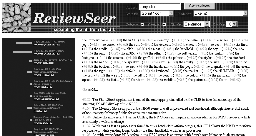
Figure 2: Initial search results screen lists categories and assessments.
Finally, we try to group sentences under attribute headings as shown in Figure 2. We attempted to use words matching the _producttypeword substitution as potential attributes of a product around which to cluster the scored sentences. although this did reasonably well (for "Amstel Light," we got back "beer," "bud," "taste," "adjunct," "other," "brew," "lager," "golden," "imported") we found that simply looking for bigrams starting with "the" and applying some simple thresholds and the same stopwords worked even better (for Amstel, we got "the taste", "the flavor", "the calories", "the best"). For each attribute, we displayed review sentences containing the bigram, as well as an overall score for that attribute. The interface also shows the amount each feature contributed to a sentence's score and the context of a sentence, as seen in Figure 3.
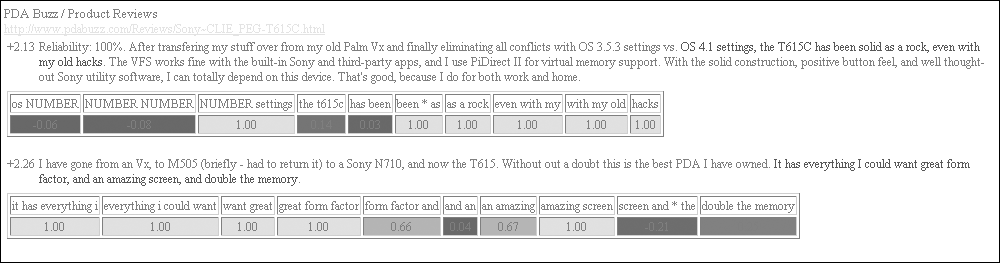
Figure 3: Screen shot of scored sentences with context and breakdown.
We were able to obtain fairly good results for the review classification task through the choice of appropriate features and metrics, but we identified a number of issues that make this problem difficult.
These challenges may be why traditional machine learning techniques (like SVMs) and common metrics (like mutual information) do not do as well as our bias measure with n-grams on the two tests. Few refinements improved performance in both cases. Encouragingly, two key innovations--metadata substitutions and variable-length features--were helpful. Coupling the _productname substitution with the best substring algorithm yielded an accuracy of 85.3 percent, higher than the 84.6 percent accuracy of bigrams. However, high variance and small sample size leaves us just short of 90 percent confidence in a t-test.
Extraction proved more difficult. It may be that features that are less clearly successful in classification, like substrings, do better in mining because they are more specific. More work is needed on separating genre classification from attribute and sentiment separation.
A variety of steps can be taken to extend this work:
[1] Yahoo! for Amazon: Sentiment parsing from small talk on the web. Proceedings of the 8th Asia Pacific Finance Association Annual Conference, 2001.
[2] Genre classification and domain transfer for information filtering. In Fabio Crestani, Mark Girolami, and Cornelis J. van Rijsbergen, editors, Proceedings of ECIR-02, 24th European Colloquium on Information Retrieval Research, Glasgow, UK. Springer Verlag, Heidelberg, DE.
[3] Good-Turing smoothing without tears. Journal of Quantitative Linguistics, 2:217-37, 1995.
[4] Predicting the semantic orientation of adjectives. Proceedings of the 35th Annual Meeting of ACL, 1997.
[5] Effects of adjective orientation and gradability on sentence subjectivity. Proceedings of the 18th International Conference on Computational Linguistics, 2000.
[6] Direction-Based Text Interpretation as an Information Access Refinement. 1992.
[7] Detecting and tracking opinions in on-line discussions. UCB/SIMS Web Mining Workshop, 2001.
[8] Automatic retrieval and clustering of similar words. Proceedings of COLING-ACL, pages 768-774, 1998.
[9] Bow: A toolkit for statistical language modeling, text retrieval, classification and clustering. http://www.cs.cmu.edu/~mccallum/bow, 1996.
[10] A model of textual affect sensing using real-world knowledge. Proceedings of the Seventh International Conference on Intelligent User Interfaces, pages 125-132, 2003.
[11] Feature subset selection in text-learning. European Conference on Machine Learning, pages 95-100, 1998.
[12] Book recommending using text categorization with extracted information. Proceedings of the AAAI Workshop on Recommender Systems, 1998.
[13] Mining product reputions on the web. KDD 2002.
[14] Thumbs up? Sentiment classification using machine learning techniques. Proceedings of the 2002 Conference on Empirical Methods in Natural Language Processing (EMNLP), pages 79-86.
[15] Beyond word N-grams. In David Yarovsky and Kenneth Church, editors, Proceedings of the Third Workshop on Very Large Corpora, pages 95-106, Somerset, New Jersey, 1995. Association for Computational Linguistics.
[16] Distributional clustering of English words. Meeting of the Association for Computational Linguistics, pages 183-190, 1993.
[17] An algorithm for suffix stripping. Program, 14(3):130-137, 1980. http://www.tartarus.org/~martin/PorterStemmer/
[18] Learning surface text patterns for a question answering system. ACL Conference, 2002.
[19] Automatically generating extraction patterns from untagged text. Proceedings of AAAI/IAAI, Vol. 2, pages 1044-1049, 1996.
[20] Affect analysis of text using fuzzy semantic typing. IEEE-FS, 9:483-496, Aug. 2001.
[21] PHOAKS: A system for sharing recommendations. Communications of the ACM, 40(3):59-62, 1997.
[22] An operational system for detecting and tracking opinions in on-line discussion. SIGIR Workshop on Operational Text Classifiation, 2001.
[23] Unsupervised learning of semantic orientation from a hundred-billion-word corpus. Technical Report ERB-1094, National Research Council Canada, Institute for Information Technology, 2002.
[24] Learning subjective adjectives from corpora. AAAI/IAAI, pages 735-740, 2000.
[25] A corpus study of evaluative and speculative language. Proceedings of the 2nd ACL SIGdial Workshop on Discourse and Dialogue, 2001.
[26] Identifying collocations for recognizing opinions. Proceedings of ACL/EACL 2001 Workshop on Collocation.
[27] Using suffix arrays to compute term frequency and document frequency for all substrings in a corpus. Proceedings of the 6th Workshop on Very Large Corpora.